Lab # 6 - FASTQ and Genome Assembly

Table of Contents

1. Introduction
2. Command Line Genome Assembly
3. Visualization
4. Galaxy

Introduction

The goal of this lab is to improve student usage of the Linux operating system and the command line, in the context Illumina FASTQ DNA sequencing data and microbial genome assembly. Students will additionally be introduced to cloud computing and the Galaxy framework for bioinformatics analyses.

Lectures - Lecture 6 slides DNA Sequencing & Genome Assembly

Flash Updates

• Illumina Sequencing
• FASTQ
• Galaxy

Demo Videos

• Using Microsoft Remote Desktop ~2 minutes
• De Bruijn graph walkthrough ~6 minutes
• Command Line Genome Assembly walkthrough ~27 minutes
• Galaxy Genome Assembly - Queuing each step ~21 minutes
• Galaxy Genome Assembly - Results ~9 minutes

Background Reading (optional)

• Myers et al. 2000. A whole-genome assembly of Drosophila. Science 287:2196-2204
• Pop. 2009. Genome assembly reborn: recent computational challenges. Brief Bioinform. 10:354-66
• Tritt et al. 2012. An integrated pipeline for de novo assembly of microbial genomes. PLoS One. 7:e42304

Computer Resources

• This lab will use McMaster's virtual Windows servers, so you need to install and set-up Microsoft Remote Desktop on your personal computer. See the demo video on how to login using Microsoft Remote Desktop and your MacID.
• All files and work on the virtual servers will be lost when you log out. Be sure to save your work elsewhere (e.g., email yourself a copy).
• Part of today’s lab will be performed at the command line and is meant to expand your linux skills. You may need your notes from the last lab as a cheat sheet. Remember, case matters for linux computers. Unless otherwise indicated, use lowercase.
• uppsala.mcmaster.ca is behind the McMaster firewall and requires VPN to connect from off campus or from the MacSecure wireless network.

Grading

• Questions are for your learning and are not graded
• Problems are worth 5 points each (-1 for each error)
• Submit your answers to the Problems, plus any supplmental multiple choice questions, on A2L Quizzes before the deadline
• An answer key to Questions and Problems will be provided on A2L after the deadline

PART 1 - Command line Genome Assembly

We are going to perform a command line assembly of a Salmonella genome that was sequenced using the Illumina platform using a kmer assembler called VELVET.

NOTE: SERVER PERFORMANCE MAY BE SLOW IF MANY STUDENTS ARE USING UPPSALA SIMULTANEOUSLY

Flash Update - Illumina Sequencing

Flash Update - FASTQ

To start:

• Log into uppsala.mcmaster.ca
• Create a new working directory for yourself (e.g. agmcarthur2)
• Move into your working directory

The FASTQ data you need is in the following files.

/home/biochem3bp3/data/Salmonella_3185_TACGAATC_L003_R1_001.fastq /home/biochem3bp3/data/Salmonella_3185_TACGAATC_L003_R2_001.fastq

Question #1. These two files contain the forward (R1) and reverse (R2) sequencing reads of this genome sequencing project. Given that the following command will tell you how many lines are in a file, how many DNA molecules have been sequenced and how many sequences are there?

wc -l /home/biochem3bp3/data/Salmonella_3185_TACGAATC_L003_R1_001.fastq

Take a look at one of the FASTQ files to remind yourself of the format and how sequencing quality is encoded:

less /home/biochem3bp3/data/Salmonella_3185_TACGAATC_L003_R1_001.fastq

We have installed software from the FASTX-Toolkit (http://hannonlab.cshl.edu/fastx_toolkit/index.html) to perform some quality control steps on these data before assembling the genome. Let’s first look at how quality varies along the sequences:

cat /home/biochem3bp3/data/*.fastq | fastx_quality_stats -Q33 -o sequences.stats

You needed to add the -Q33 parameter to tell it that you're using Illumina encoded quality scores, not Sanger encoding. First take a look at the contents of sequences.stats using the command line and then download the pre-calculated EXCEL spreadsheet in A2L/GitHub to view on your computer. You can find a key to the column labels here: http://hannonlab.cshl.edu/fastx_toolkit/commandline.html#fastq_statistics_usage

Question #2. Looking at the plot, we want trim the reads where the average quality becomes worse than a 1 in 100 error rate (Q20). At what position along the read on average would you trim the data?

Now trim the reads by length using the following command, but replace the word POSITION with the value you decided above (-f is first position to keep, -l is last position to keep):

cat /home/biochem3bp3/data/*.fastq | fastx_trimmer -Q33 -f 1 -l POSITION > sequences.trim

We now want to additionally clip and filter the reads. The clipping removes the synthetic Illumina DNA adaptor sequence TACGAATC while the filter removes any reads of length less than 32 bp after removal of the adaptor. We pick 32 bp as when we assemble we will be using 31 bp kmers. The -v is for verbose mode, giving a summary of the results.

fastx_clipper -Q33 -l 32 -v -a TACGAATC -i sequences.trim -o sequences.clip

Question #3. How many sequences passed this filter?

Lastly, we want to perform a quality filter, such that we only keep sequencing reads for which at least 95% of bases are Q20 or better:

fastq_quality_filter -Q33 -q 20 -p 95 -v -i sequences.clip -o sequences.filter

Question #4. How many sequences passed this quality filter?

Now look at the results to see how the data have changed:

less sequences.filter

The original data were paired reads (i.e. forward & reverse) but some of the pairs may have been lost by the filtering. The Velvet assembly algorithm treats paired and unpaired reads differently as only the former can create scaffolds, so we need to put these in different files using one of Dr. McArthur’s Perl scripts:

fastq_interleave sequences.filter
ls

Question #5. How many paired and unpaired reads are in the final pre-assembly data?

Question #6. This strain of Salmonella is expected to be ~4,600,000 bp in size. What base pair coverage are we about to submit to the Velvet assembly?

We are now going to use the Velvet assembly to make contigs and scaffolds. First we need to make an assembly directory and then calculate the kmers present in the sequencing reads. The Velvet algorithm requires the kmer value to be an odd number to avoid palindromes. Longer kmers bring more specificity, but lower coverage. The Velvet package has been found to perform well with kmer length of 31 bp:

Something went wrong above and you need correct results for the VELVET assembly? Type "cp ../result/* ."

mkdir draft_assembly
velveth draft_assembly 31 -fastq -shortPaired sequences.filter.paired -short sequences.filter.unpaired

With the kmer sequences and their frequencies now calculated, we can have Velvet determine the de Bruijn graph for these sequencing reads and use the Eulerian path to resolve contigs. The paired reads will then be used to create scaffolds among the contigs. We are going to let the Velvet assembler determine the expected kmer coverage from the data itself and thus determine the minimum coverage cut-off for forming contigs. Once the assembly is done, we will use one of Dr. McArthur’s Perl scripts to summarize the results:

velvetg draft_assembly -cov_cutoff auto -exp_cov auto
scaffoldstats draft_assembly/contigs.fa

Question #7. If you browse through the output, how many kmers were found in the sequencing data?

Question #8. What fraction of the sequencing reads contributed to the final assembly?

Question #9. The Final Graph in Velvet refers to the contig sequences, whereas the output of scaffoldstats refers to scaffolds. Is the N50 higher for the scaffolds than the contigs? Why?

Question #10. Why is the final estimated coverage lower than what we estimated in Question 6?

Record some statistics for later comparison:

• Total number of scaffolds:
• Total scaffold assembly length (bp):
• Scaffold N50 (bp):
• Largest scaffold (bp):

Visualization

We now want to visualize our assembly instead of just looking at statistics. Some of these results are pre-computed screenshots since the analyses are not quick and we are going to learn the details of Burrow's Wheeler Transform next week.

Visualizing BWT read mapping was performed using Tablet, https://ics.hutton.ac.uk/tablet/

We use the Burrows-Wheeler algorithm (BWA) to align our raw sequencing reads to the assembled contigs so we can see where each read contributed to the final assembly. Usually, BWA is used to align NGS sequences to a reference genome, such as the published human genome. In this case, we are using the contigs as the reference genome. Visualizing reads that aligned to the contig Node 1:

Zoom of above image to show agreement (and rare disagreement) among sequencing reads. The disagreement could be true polymorphism or sequencing errors:

Visualizing similarity between assembly and a reference Salmonella genome was performed using MAUVE, http://darlinglab.org/mauve/mauve.html

Comparison of the assembly contigs (bottom) to the complete genome sequence of a reference Salmonella strain (top). Blocks reflect regions of shared sequence, red lines gaps:

Lastly, using the lab computers, visualize the quality of the assembly graph, with an emphasis upon repeated sequences, using BANDAGE (https://rrwick.github.io/Bandage) and the LastGraph.txt file available on A2L/GitHub.

Problem #1. Based on the Tablet, MAUVE, and BANDAGE results, what is your assessment of the quality of your genome assembly?

PART 2 - Galaxy

Flash Update - Galaxy

Today’s lab will use the public server of the Galaxy project, http://usegalaxy.org. It is used by thousands of researchers, so you will be sharing computational resources – not all steps will perform quickly. Use the following steps to set up your account:

• From the top menu of the site, select Log in or Register and register for an account. This is your free account on the most complete and most maintained Galaxy server – use it whenever you have genomics data!
• Check your email account for a message from the server and confirm you registration. This must be completed before the server will analyze your data.
• Return to the Galaxy home page.

The walkthrough video provides a demonstration of the Galaxy workflow environment and will assemble a Salmonella genome sequencing project which will be used in next week’s molecular epidemiology laboratory.

If you are new to Galaxy, you will have an empty Unnamed History. Otherwise, use the plus sign to create a new History. Either way, give your History a name:

Upload the lab data below via the Upload Data tool's Paste/Fetch option. There are two ways you can do this:

• Download the two files below and then upload them to Galaxy (very slow)
• Use the URLs from the files below (recommended, fast, see screenshot below)

Salmonella_3185_TACGAATC_L003_R1_001.fastq.gz

Salmonella_3185_TACGAATC_L003_R2_001.fastq.gz

These are the forward and reverse FASTQ read files for a Salmonella assembly data set. The data files will show up on the right panel in green when you succeed in uploading them. By click on the file name you will expand the green box to see all the contents. The eye icon at the top will show the contents on the main screen. The i icon in the middle of the green box will show the file and analysis details, including STDOUT (important!).

Galaxy Hints: Green = Done, Yellow = Running, Red = Error, Gray = Queued

FASTQC

You will be shown how to use the FASTQC tool. Run FASTQC on both data files using the default settings and you will generate raw and web page results for both files.

See the FASTQC Documentation and video tutorial.

Here is an example of the Per base sequence quality from another data set:

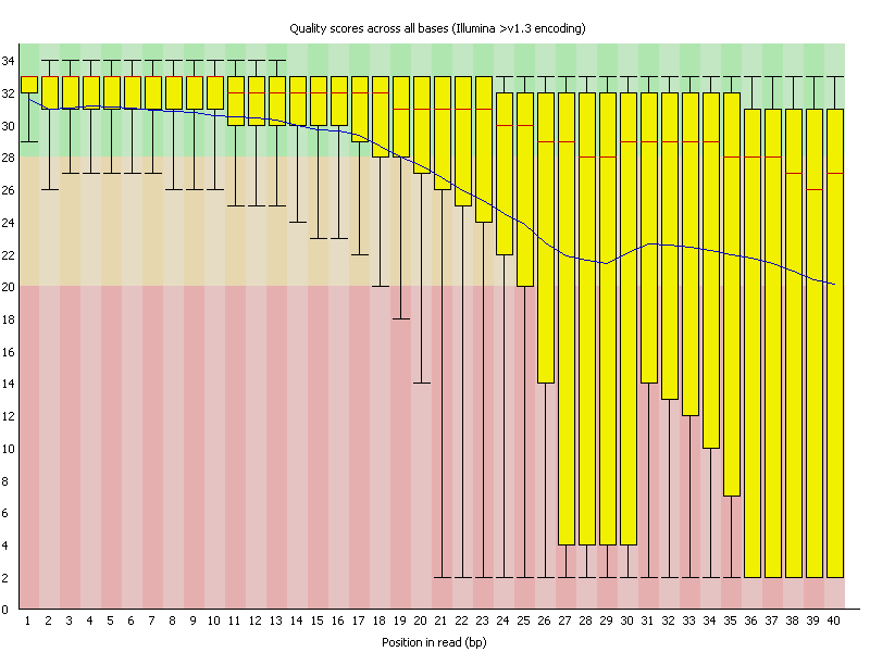
For each sequenced nucleotide (start of read to end of read) a BoxWhisker type plot is drawn. The elements of the plot are as follows:

• The central red line is the median value
• The yellow box represents the inter-quartile range (25-75%)
• The upper and lower whiskers represent the 10% and 90% percentiles
• The blue line represents the mean quality

The y-axis on the graph shows the quality scores. The higher the score the better the base call. The background of the graph divides the y axis into very good quality calls (green), calls of reasonable quality (orange), and calls of poor quality (red). The quality of calls on most platforms will degrade as the run progresses, so it is common to see base calls falling into the orange area towards the end of a read.

Question #11. In your Salmonella data, at what position along the reads does the mean quality fall below Q20? Is it the same for both the forward and reverse reads?

Question #12. After reading the documentation on the FASTQC plots, do you think there is any evidence that the sequence library is biased (i.e. non-random)? Explain your reasoning.

FASTQ GROOMER

The FASTQ data is in Sanger / Illumina 1.9 format but needs to be in standard Sanger FASTQ format for downstream steps. Use the FASTQ GROOMER to convert the data to Sanger FASTQ.

TRIMMOMATIC

You will be shown how to use the TRIMMOMATIC tool to perform quality trimming on your data. Run TRIMMOMATIC on both groomed data sets (including ILLUMINACLIP, but everything else default):

Trimmomatic will separate the data into paired and unpaired reads, just like our steps in the linux assembly above. Ignore the unpaired reads and only used the paired reads going forward. Take a look at the new FASTQ files and then analyze the groomed and trimmed paired reads using FASTQC.

Question #13. How does the trimmed FASTQ data differ from the original FASTQ data? How will the trimming improve your assembly?

PREPARING FOR ASSEMBLY

Just like the fastx_trimmer tool we used at the command line, TRIMMOMATIC may have removed some poor quality sequences, putting the forward and reverse FASTQ files out of sync. First use the FASTQ Interlacer to merge all of the paired data into one file

Next, use FASTQ De-Interlacer to split the resulting file into Forward, Reverse, and Orphan reads. Almost all assemblers required FASTQ data sorted in this manner to save on initial preprocessing. The most common reason for a failed assembly is skipping this step.

UNICYCLER ASSEMBLY

At the command line we used the older assembler VELVET and in the lecture we learned about the all-in-one microbial assembler A5. We are going to perform our final assembly using the Unicycler assembler, which is considered the best for kmer based assembly. Unicycler has powerful defaults, so perform the Unicycler assembly using the FASTQ De-Interlacer results and without changing any of the parameters, except for:

• The forward reads should be the FASTQ De-Interlacer left mates
• The forward reads should be the FASTQ De-Interlacer right mates

VISUALIZATION AND STATISTCS

Unicycler will create two output boxes, one containing the assembly graph and they other the contig FASTA sequences. Download the Unicycler assembly graph file and use BANDAGE (https://rrwick.github.io/Bandage) to visualize the assembly.

We can also use the Quast tool to generate assembly statistics, reading the PDF report to view the assembly statistics:

• Set mode to Individual Assembly

INTERPRETATION

By the end of the lab, you should have all of the steps in the Galaxy que. Once they are all complete, using the Quast results and the BANDAGE plot to answer the following questions:

Problem #2. Based on the statistics above, do you think this is a high quality assembly of a Salmonella genome? Explain your reasoning.

Problem #3. Compare this assembly to the command-line Velvet assembly. The Unicycler assembly had more FASTQ data and a better algorithm, but what specifically improved in the assembly?